Processing Images

Assumptions

1. A sequence of images has been captured with the HQ-camera at time instances {t₁, t₂, …, t_n, …} where time instances increase with t_n-1 < t_n < t_n+1.
   1. each time instant t_n corresponds to an image I_n
2. A fixed camera position is used for all images.
3. The scene may change over time however and we are interested to detect such changes:
   1. changes may occur due to time varying lighting conditions
      1. using a small duration Dt = t_n – t_n-1 should result in quasi-constant lighting conditions between image captures
   2. objects may enter or leave the scene or move within the scene

Goals

1. Detect whether the scene has changed (motion detection) between adjacent time instants.
2. Perform some experiments to explore these subjects. To this end an Ipython notebook has been set up demonstrating the procedure. The following section highlights the main steps.

Motion detection / Principles

For details of the implementation consult the Ipython notebook. (see embedded document or download)

Experiment#1

The same scene has been captured with the HQ-camera module and saved to files with different methods:

1. image has been captured directly into a file as a compressed image (jpeg) : image: img1
2. image has been captured as array (ndarray object) and save to file as jpeg (using OpenCV): image: img2
3. image has been captured as array (ndarray object) and saved to file (no compression): image: img3

Images are then retrieved from files and stored in ndarray objects.

Since we have 3 images (img1, img2, img3) taken from the same scene with unchanged camera position these images should look identical as is shown in the next figure.

Later it is demonstrated however that each image is slightly different depending on how it has been captured and stored to a file.

An image captured to a ndarray and saved to file using numpy.save() method is a “lossless” representation of the captured image since it has not been compressed before saving it. On a per pixel basis such image must be different to images which have been captured and compressed before storing them.

But even for two images which have been captured in a compressed format (see method 2 and 3) small differences should be expected. (method 2 used OpenCV to compress to jpeg while method 3 used the built-in codec of the camera)

And even if we had captured two consecutive images in a lossless format (numpy) these images would be still be slightly different due to the additive noise added by the camera’s sensor during capturing these images.

Therefore when deciding whether images are identical (almost identical) or significantly different, the effect of noise in images must be taken into account.

To compare these (almost) identical images, some pre-processing of images must be done. Here a simple method is used to show the principle. Very likely this method needs to be improved to result in a fairly robust approach to compare images reliably.

step 1)

From the original images img1, img2, img3 blurred versions of images have been created. Here we apply gaussian blurring. All images have been converted to gray-scale images before blurring/smoothing them. After blurring, images are denoted img1_blur, img2_blur, img3_blur.

step 2)

Take absolute difference (absdiff) images. Since we have 3 images there are 3 image pairs to consider when computing absolute differences:

img1_2 := absdiff of images (img1_blur, img2_blur)

img1_3 := absdiff of images (img1_blur, img3_blur)

img2_3 := absdiff of images (img2_blur, img2_blur

step 3)

Apply binary thresholding to absdiff images img1_2, img1_3, img2_3. Every pixel is set to 0 if absdiff is below threshold. Otherwise set to maximum (255). As a result we get thresholded images with binary pixel values (0: black, 255: white). These thresholded images are denoted img1_2_th, img1_3_th, img2_3_th and are shown in here:

Apart from a few white pixels all three absdiff images are black (pixel value: 0) indicating quasi-identical images.

Having shown that the procedure works at least for almost identical images we are now going to appy it to images which are known to be different.

Apart from a few white pixels all three absdiff images are black (pixel: 0) indicating quasi-identical images.

Having shown that the procedure works at least for almost identical images we are now going to appy it to images which are known to be different.

---

Experiment#2

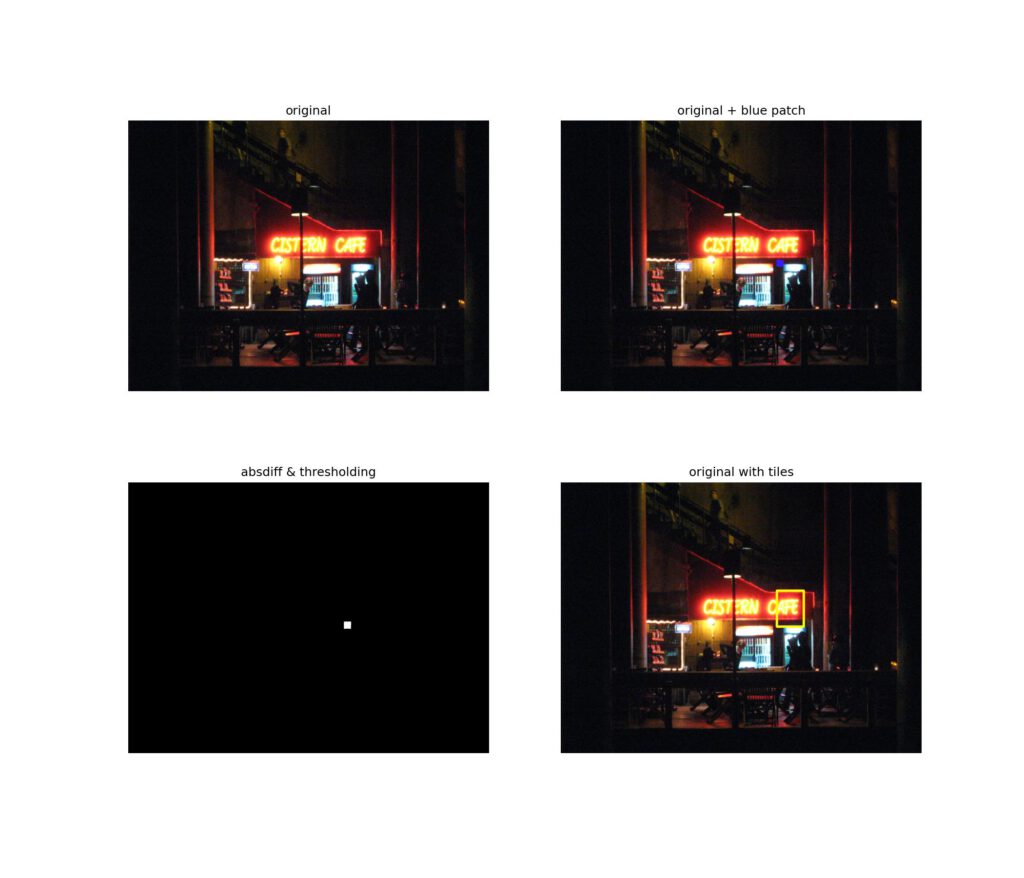
We compare two images. The original image is from a photograph. The second image is derived from the original image by adding a small square blue patch on it. In the figure below the original image and derived image are shown on the upper left and upper right of the figure.

Converting these images to gray-scale before burring, taking absdiff and applying a threshold results in a binary image shown on the lower left of the figure. (The blue patch has been turned into a white patch in this figure.)

Finally we partition/tile the image on the lower left into a number of non-overlapping sub-images. For each sub-image the number of non-zero pixels is counted. The ratio of non-zero pixels vs. the total number of pixels of the sub-image provides a measure indicating the mismatch in this sub-image (the larger the ratio the more likely it is to have significant mismatch). Selecting sub-images where this ratio exceeds some user defined threshold helps us identify those parts where the original image and the modified image show larger deviations which are (most likely) not due to noise. The image on the lower right shows the original image which such regions of interest marked by rectangular frame with yellow border.

---

Experiment#3

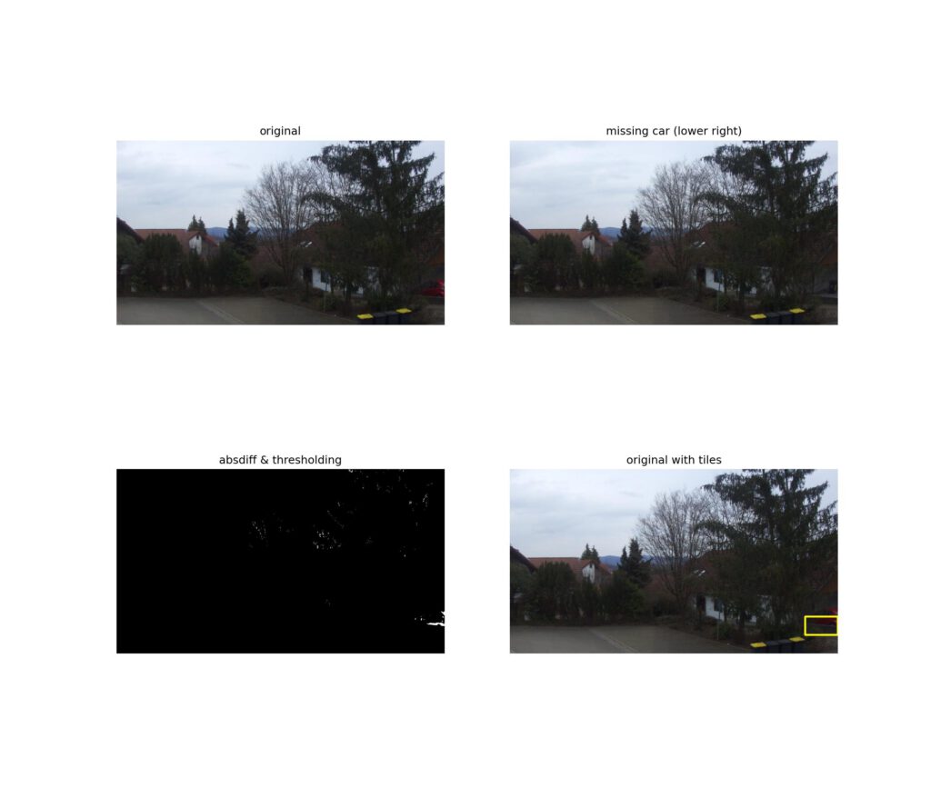
Here we repeated experiment#2. This time the upper left and upper right images of the next figure are compared. Apart from noise and possibly slight deviations in lightning conditions the main difference is that a red car on the lower right of the figure is missing in the upper right image. The contrast is quite poor so the difference is barely noticed at first glance.

Applying the same procedure as described for experiment#2 the missing car on the upper right image is detected and highlighted by a yellow frame on the lower right image of the figure:

---

Summary

To detect differences of two images the absdiff method (see OpenCV) and thresholding have been used to remove the common background of two images. Future work must be directed to implement a more robust method of background removal and feature detection to create a “production quality” detector that can reliably detect changes between images. A promising approach would be to detect features (edges, corners, shapes, etc) of each image. In a second step the comparision is done on the basis of these features.

Currently however I will stick with the method presented here. It is simple and fast enough to be implemented on the Raspberry Pi. Above all it is easy to understand.

Going further requires to learn more about computer vision and image processing techniques. I would rather like to go in this direction but obviously this is fairly time consuming if you do not just want to apply recipes.

---

Resources:

https://docs.opencv.org/4.x/d6/d00/tutorial_py_root.html

https://pyimagesearch.com/2014/09/15/python-compare-two-images/

books:

Consise Computer Vision; Reinhard Klette; Springer

Programming Computer Vision with Python; Jan Erik Solem